Fewer clues can help a model generalize. Not every change is safe.

Can a model get the answer right on unfamiliar examples? That ability is called generalization. This paper asks when a rule that uses fewer clues can keep working after the examples change.
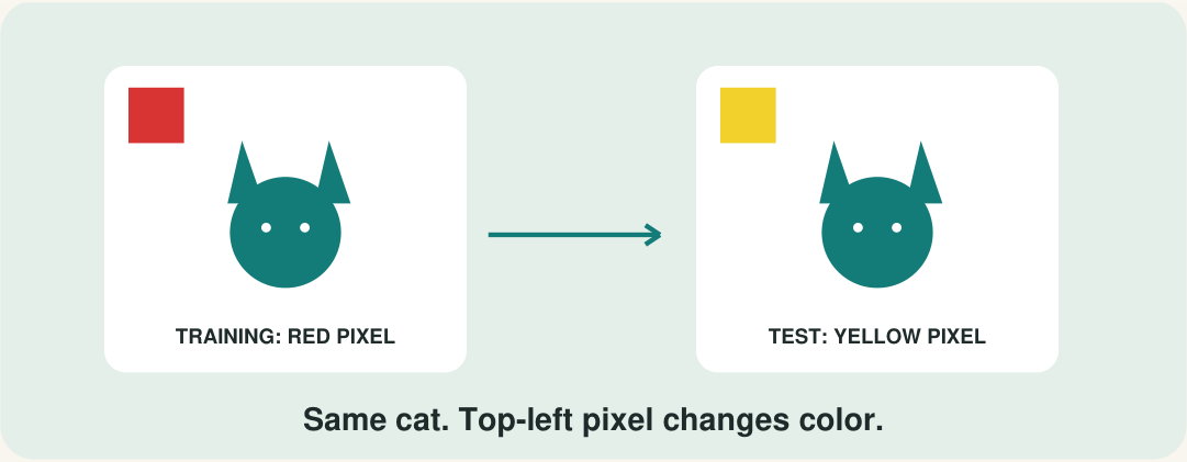
Changing a pixel's color does not change which animal is in the photo. But correct training answers do not tell us which rule the model learned. Does it name the animal regardless of pixel color, or change its answer when that color changes?
Explained simply
A rule that ignores a clue cannot be affected by changes to that clue. The catch: we must check what the model actually uses, not what we think it should use.
What you will learn
- How a model can get the right answer for the wrong reason.
- Which clues must stay familiar when other things change.
- How to test whether an unnecessary clue changes the answer.
Paper: Scott Aaronson, Lin Lin Lee and Jiawei Li, researchers at the University of Texas at Austin. Sparsity and Out-of-Distribution Generalization asks when rules using few clues can work on unfamiliar examples.
Read the original paper. The cat/dog and red/yellow pixel example is on page 2. The cover redraws the idea with simple icons and enlarged color squares. It does not show an experiment.
01. Two rules can pass the same test
What did the model learn from those cats and dogs? Training photos are the examples used to teach it. Imagine they all have a red top-left pixel, and the model names every animal correctly. Two different rules could explain that success.
A feature is a clue in the information given to a model. Here, the animal is the clue that should decide the answer. The pixel color is another clue. This is a simplified example. A real model may need many image details to recognize an animal.
One rule names the animal and ignores the pixel. Another names it correctly when the pixel is red. When the pixel is yellow, that second rule calls a cat a dog and a dog a cat. Both rules get every red-pixel training example right.
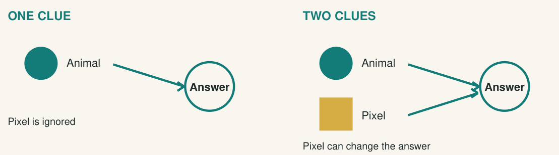
Testing on new photos can still miss the problem. If those photos also have red top-left pixels, both rules pass. Now try yellow pixels. That creates a distribution shift, a change in the examples the model sees or how often each kind appears.
Other ways to tackle this problem We could teach the model with more varied photos, change background details while it learns, or discourage overly complicated rules. This paper does not compare those methods. It asks: what conditions let us prove that a learned rule will still work on changed examples?
The example comes from page 2 of the paper. The diagram shows which clues each rule uses. It does not show measured results.
02. Simple means fewer clues, not fewer words
The two rules passed the same training test. To tell them apart, the authors count how many clues each uses. They call using few clues sparsity. A k sparse rule uses no more than k clues. If k is 2, that means at most two. Our animal rule uses one; the pixel rule uses two.
This follows Occam's razor, the idea of favoring simpler explanations. Here, simpler means using fewer clues, not fewer words. It also differs from using fewer parameters, the internal numbers adjusted during training. A model with fewer parameters could still use many clues.
The paper gives another example: emeralds, the green gemstones. One rule says they stay green. Another says they are green before a chosen date and blue afterward. Before that date, both agree with what we see. The second rule uses an extra clue: time.
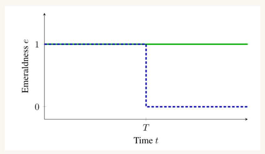
Figure 1, from the paper. Read time from left to right. The height of each line stands for a color, not a measured amount. The green line always says green. The blue dashed line changes its answer at T, the chosen date. Before T, both rules agree. Original Figure 1.
Credit: Aaronson, Lee and Li, arXiv:2603.07388v1, Figure 1. Reproduced from the PDF; no data or plotted lines changed.
But what counts as one clue depends on how the input is described. Coordinates are the separate numbers in that description. Combining those numbers can change how many coordinates a rule uses. The next section explains how the authors describe simple rules without relying on that choice.
03. What must stay the same
Counting clues gives us a preference, not yet a guarantee. The paper adds a theorem, a statement proved mathematically. It requires a condition on every clue used by either the correct rule or the learned rule: each combination of these clues must be equally likely in the training and test data.
A joint distribution describes combinations of clues and how likely each is. Checking clues separately can miss a change. For example, in each of two photo sets, half the animals are cats and half the top-left pixels are red. Red could appear only in cat photos in one set and only in dog photos in the other. This is a teaching example.
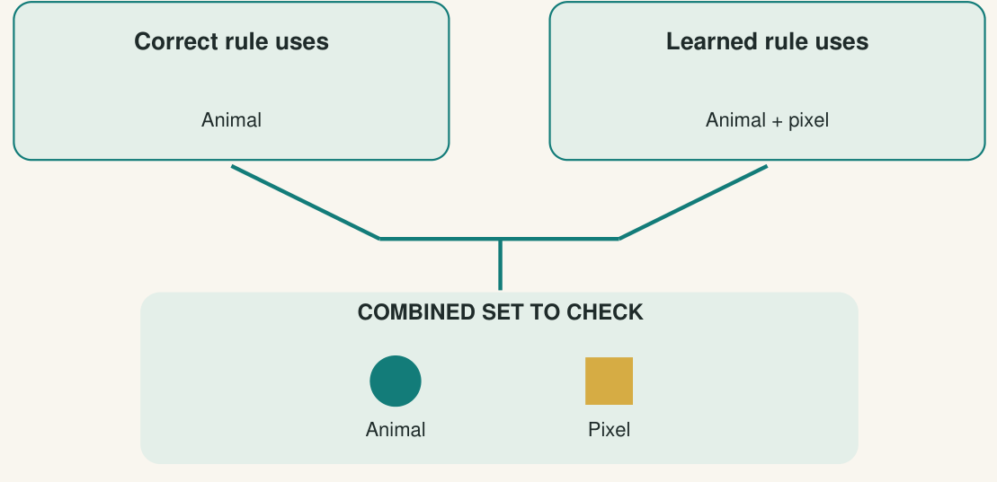
If both rules use only the animal, we check only that clue. Pixel changes cannot affect either answer. If the learned rule also uses the pixel, we must check both clues together. Turning red pixels yellow breaks this condition. This proof no longer promises success.
An unnecessary clue can still matter to the model. Calling it irrelevant does not prove that the model ignores it.
The proof also requires
- Both rules belong to the specified group using at most k clues.
- Enough examples, drawn from the training data pattern without one draw affecting another.
- A limit on how flexibly the allowed rules can assign answers.
- A learned rule that gets every training answer right. For most independently drawn training samples, the rate of future mistakes stays below a chosen limit. Some samples can still fail.
Source: Theorem 3. Theorem 4 also covers unequal probabilities, if a mistake that is common at test time is likely enough to appear during training. The required sample size depends on that overlap.
04. Why an unused clue can change
The condition checks only the clues those two rules use. That still leaves room for big changes elsewhere. Suppose both rules use only which animal is shown. The wallpaper, camera marking and pixel color can all change. If cats and dogs still appear just as often, those unused details do not affect either rule.
Whether an answer is wrong depends only on the clues used by the learned rule and the correct rule. If both ignore a clue, changing it cannot create a mistake. The rest of the proof limits mistakes on the clues they do use.
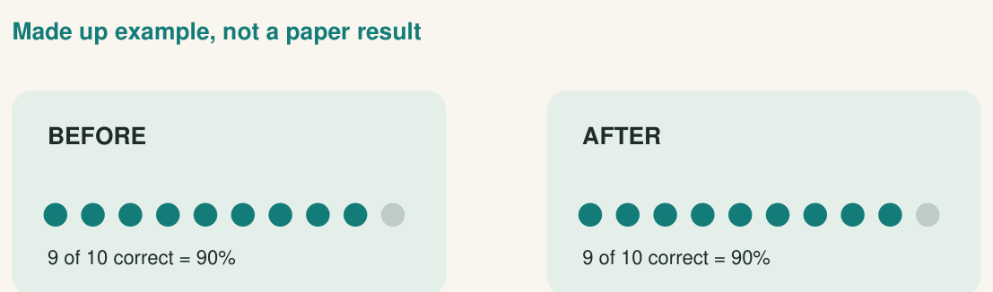
These dots show ten made up examples. Nine correct answers out of ten is 90%. Now change only a pixel that the rule ignores. Every answer stays the same, so the score stays 90%. This is invariance, unchanged behavior after a particular change. No real model was tested here.
Real models can combine input numbers before using them. The authors study a subspace junta, a rule using a few weighted sums of those numbers. A weighted sum multiplies each number by a chosen weight and adds the results. Each sum can include many input numbers.
As a teaching analogy, rotate a map. North no longer points to the top of the page, but the map describes the same place. Similarly, rotating the way input numbers are represented need not make a rule more complex. The authors want their definition of simplicity to survive that change.
Even one weighted sum is not enough: changing its weights can create a very flexible family of
rules (Claim 1). The paper needs a limit on the whole family's flexibility. Without that limit, finitely
many training examples need not be enough.
05. What this does not prove
We now have two limits: which clues the rules use, and how flexibly the rules can assign answers. These conditions matter. The proofs do not show that today's language models, systems that generate text, work safely on unfamiliar examples. The paper connects its question to AI alignment: getting an AI to keep behaving as intended.
A model could behave well while it learns and differently after release. It might use a clue that tells it which setting it is in. If so, that clue matters to its rule. We cannot treat changes to it as harmless just because the model should ignore it.
The paper gives sufficient conditions: conditions that would make its guarantee apply. It does not show that real systems meet them. Nor does it show that we know all their clues or that a practical training method will find a rule using few clues.
Keep these limits visible
- A small model does not necessarily use few clues.
- Getting training answers right does not show why they were right.
- Clue counts can match even when clue combinations differ.
- A proof about rules that choose between two answers does not guarantee safe text generation.
- This paper gives proofs, not measured accuracy improvements.
This question connects to earlier posts, but is different. One asks which answers get credit during training. Another asks which problems get more practice. This paper asks whether the rule still works when the examples change. Answering one question does not settle the others.
Previously covered
A coin flip made this model better at math. Or did it? asks whether the feedback used during training explains why a model improved.
Your model found the right answer. It might never learn to find it again. explains why getting an answer right once is different from learning to get it right again.
06. What I tested: a small shortcut diagnostic
The paper's guarantee depends on which clues a rule actually uses. Checking one clue at a time may not tell us enough. A wrong rule could fail only when several clues change together.
This diagnostic is a small demonstration of what checks can miss, not a new learning method. The comparison below was run over handcrafted rules. No model was trained.
The diagnostic, explained simply
Imagine 12 switches that can be off or on. Only the first two decide the answer. If they match, the answer is 0. If they differ, the answer is 1. The other ten should make no difference.
I added deliberately wrong rules that reverse the answer when a particular combination of the other switches appears. Then I compared ways of finding those traps and scored the surviving rules on every setting.
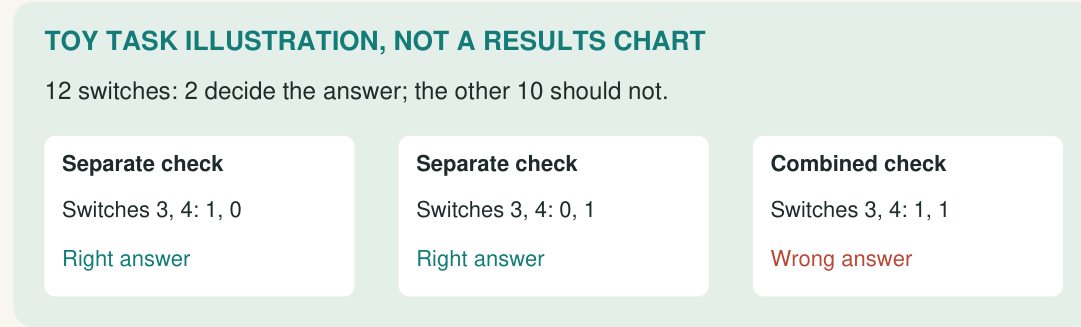
In this illustration, a wrong rule reverses the answer when switches 3 and 4 are both on. Turning either on alone misses the mistake. Turning both on reveals it. Off is 0 and on is 1.
Build the starting rules
Use all 44 training rows: the four settings of the first two switches, each combined with the 11 extra-switch settings that have either none or just one on. These are examples each candidate rule must answer correctly, not a model-training run.
Keep the correct rule. For each chosen subset of two, three or four extra switches, add a rule that reverses the answer whenever those switches match a chosen off/on pattern. Include patterns containing at least two on switches. Switches outside the chosen subset do not affect that trap.
Every trap is absent from training. All these wrong rules therefore pass the 44 rows. This is deliberate: it creates a controlled blind spot, not evidence that real models commonly learn these rules.
06. The checks I compared
An audit is a set of answer checks used to reject wrong rules. The comparison has three selection methods plus one deliberately ineffective control.
| Method | How it chooses checks | What it knows |
|---|---|---|
| One-switch control | Replays training rows with one extra switch on. Zero new evidence. | Input settings only |
| Random combinations | Uniformly draws unused settings from the 1,013 extra-switch combinations absent from training. | Input settings only |
| Pair coverage, then fixed order | First covers missing pair assignments; once covered, chooses by binary order. | Input settings only |
| Rule disagreement | Chooses a setting where the surviving rules split their predictions most evenly. | The full candidate list and its predictions |
Why the control cannot help
Every one-switch check is already a training row. Every candidate already passed it. Replaying these rows rejects no new rules. This is a negative control, an intentionally ineffective check, not a competitive method.
A solved reference case, not an experimental discovery
Separately, list every rule using at most two switches and keep those that fit all 44 training rows. Only the correct first-two-switch rule survives. An exhaustive check of every two-switch answer table confirms this. Its error is zero on this toy task before any audit.
This demonstrates what an imposed clue restriction buys in this exact setup. It does not show that a model can learn that restriction, or that a small model uses few clues.
What the comparison measures
The comparison asks which checks reject more hidden traps for a fixed answer-check budget. It does not test the paper's theorem. The pair method has a special limitation: training already covers 135 of the 180 pair assignments. Its first all-on row covers the remaining 45, so every later choice is fixed-order selection.
06. Make the comparison reproducible
One row means one answer check
Use limits of 8, 32 and 128 complete 12-switch rows. Each row costs one checked answer. Do not multiply a row into four checks without counting them. Select each row before revealing its correct answer, then remove candidates that answer incorrectly.
The three active methods choose only settings absent from training. There are 1,013 possible extra-switch settings: 1,024 total minus the 11 already covered. Within a run, never reuse an extra-switch setting, even with different useful switches.
Exact selection rules
- Random selection: draw uniformly without replacement from those 1,013 settings. Repeat 20 runs with fixed starting numbers 0 through 19 for the random-selection software. The run used NumPy 2.2.6 and Generator(PCG64(seed)).choice, one uniform draw from the ascending list of remaining settings at a time. Python was 3.10.12. The 8, 32 and 128 limits were checkpoints of the same run for each seed. Report the mean and range of the measurements.
- Pair coverage, then fixed order: there are 45 pairs among ten extra switches, each with four assignments, 00, 01, 10 and 11. Mark assignments seen in training as covered first. At each step, choose an eligible setting that adds the most uncovered pair assignments. If all assignments are covered, use the fixed order below.
- Rule disagreement: among eligible rows, choose the one that makes the surviving rules split their 0 and 1 predictions as evenly as possible. Equivalently, maximise the smaller of those two counts. If only the correct rule remains, stop.
- Balance the useful switches without extra queries: on successive checks use 00, 01, 10, 11, then repeat. The chosen extra-switch setting is combined with just that step's useful-switch setting.
- Break every selection tie by increasing binary value of the ten extra switches, reading switch 3 first as the highest-place digit. Repeat random runs only; the other methods are deterministic under these rules.
Matched answer checks, not matched total work
The control follows the same 00, 01, 10, 11 useful-switch cycle, first with switch 3 on, then switch 4, and so on through switch 12. It stops after those 40 distinct training rows. Record checks used and new rows separately: the control always has zero new rows. Active methods have one new row per check.
Rule disagreement gets privileged access to the handcrafted candidates. Report selection time and number of candidate predictions inspected separately from answer checks. A win under the same answer-check limit is not automatically a win in total cost.
07. How I scored the checks
Score only after selection finishes
Twelve switches give 4,096 settings. Evaluate every surviving rule on all of them only after the audit. Do not use those scores to choose checks. Each setting gets equal weight: this is a uniform-grid diagnostic, not a measure of deployment risk.
| Measurement | Plain meaning |
|---|---|
| Worst surviving error | Largest wrong-setting fraction among surviving rules. Denominator: all 4,096 settings, equally weighted. |
| Missed-rule share | Surviving wrong rules divided by the original wrong-rule count. Count distinct full answer tables once. |
| Checks to remove every trap | Record the first check at which no wrong rule remains, within the largest 128-check run. If none does, report not eliminated within the actual checks performed. |
| Work and new evidence | Record checked rows, rows absent from training, candidate predictions inspected and selection time separately. |
Report two-, three- and four-switch traps separately. The correct rule always survives, so the worst-error measurement remains defined even when all wrong rules are rejected.
Size of the demonstration
| Trap uses | Possible reversal patterns |
|---|---|
| 2 extra switches | 45 |
| 3 extra switches | 480 |
| 4 extra switches | 2,310 |
| Total before removing identical rules | 2,835 |
For each chosen subset, keep only patterns with at least two on switches. The counts are 45 × 1, 120 × 4 and 210 × 11. At 4,096 answers per reversal rule, the tables contain 11,612,160 entries. One byte per answer uses about 12 MB, plus working memory. No large model training is needed.
07. What happened when I ran it
Start with 2,835 wrong rules. Lower survivor counts mean fewer traps slipped through. These are measured results from this finite diagnostic, not results from the paper.
| Method | 8-check limit | 32-check limit | 128-check limit |
|---|---|---|---|
| One-switch control | 2,835 | 2,835 | 2,835 (40 used) |
| Pair coverage, then fixed order | 2,266 | 1,908 | 1,330 |
| Rule disagreement | 1,035 | 0 (31 used) | 0 (31 used) |
| Random, 20-run mean | 1,510.15 | 273.9 | 0.25 |
| Random, run range | 1,150 to 1,865 | 164 to 483 | 0 to 2 |
Fractional counts in the random row are averages, not fractional rules. Each individual run has an integer survivor count. Checkpoints report the state after up to the stated limit; methods stop if all wrong rules are gone.
The failure that an average can hide
Random checks found every trap within 128 checks in 17 of 20 runs. Seed 1 still left one four-switch trap; seeds 4 and 12 left two each. Each survivor gets 6.25% of the uniform grid wrong. A mean of just 0.25 surviving rules must not be read as guaranteed success.
Among the 17 successful random runs, the first complete elimination took 83 to 124 checks. The other three are not eliminated within 128. The one-switch control removed nothing in its 40 actual checks. Pair coverage followed by fixed order still left 1,330 wrong rules after 128.
Which trap sizes survived?
| Method and limit | 2-switch | 3-switch | 4-switch |
|---|---|---|---|
| Control, any limit | 45 | 480 | 2,310 |
| Pair then order, 8 | 0 | 320 | 1,946 |
| Pair then order, 32 | 0 | 256 | 1,652 |
| Pair then order, 128 | 0 | 168 | 1,162 |
| Disagreement, 8 | 0 | 36 | 999 |
| Disagreement, 32 or 128 | 0 | 0 | 0 |
| Random mean, 8 | 4.2 | 156.85 | 1,349.1 |
| Random mean, 32 | 0 | 5.9 | 268 |
| Random mean, 128 | 0 | 0 | 0.25 |
Disagreement eliminated every two-switch trap at check 1, every three-switch trap at check 10, and every four-switch trap at check 31. Pair coverage eliminated all two-switch traps at its first check, but not all larger traps within 128.
07. What the results do and do not mean
Worst surviving error, not just survivors
| Method | After 8 checks | At 32 limit | At 128 limit |
|---|---|---|---|
| Control | 25% | 25% | 25% |
| Pair then order | 12.5% | 12.5% | 12.5% |
| Disagreement | 12.5% | 0% | 0% |
| Random, across runs | 12.5% to 25% | 6.25% to 12.5% | 0% to 6.25% |
Zero here means the correct rule is the only surviving candidate on this finite grid. It is not a safety claim about models or other inputs. All of these errors weight the 4,096 settings equally.
What is already known
Each individual two-, three- or four-switch trap reverses the answer on exactly one quarter, one eighth or one sixteenth of this uniform grid. Those are consequences of construction, not experimental results. The measured comparison tracks which traps survive the chosen checks.
Why disagreement won this comparison
Disagreement could inspect the entire handcrafted candidate list, choose informative rows and remove rules after each answer check. Finding all listed traps in 31 checks in this implementation involved inspecting 21,889,911 candidate predictions during selection. That work is separate from the 31 answer checks; this is not proof of lower total cost.
The pair method is weaker here for a specific reason: one all-on row completes pair coverage. Its later checks follow binary order, not remaining pair gaps. This result does not establish that pair-guided testing is generally worse than random testing.
A solved reference, kept separate
The at-most-two-switch restriction leaves one correct rule, zero wrong rules and zero audit queries. That was verified by enumeration before the comparison. It shows what the imposed restriction guarantees in this construction, not what a model learned.
Reproduce this run
The accompanying Python script includes all 2,835 reversal rules, full 4,096-setting scoring, query histories and seeds 0 through 19. Run with Python 3.10.12 and NumPy 2.2.6. Uniform random choices are sequential, without replacement, over ascending remaining settings. Limits 8, 32 and 128 are prefixes of one run per seed.
An independent replay of the saved query histories agrees with every survivor count. Only diagnostic properties and audit outcomes were computed. The broader image and assistant applications below remain suggestions.
07. Where this could be useful, and where it stops
The switches stand in for clues a model might use. These are possible applications of the checks, not experiments demonstrated by the paper or by this toy run.
- For an image model, keep the animal the same but change background and lighting together. For an assistant, keep the request's meaning the same but change wording and formatting together. First confirm that the correct answer should not change. A newly wrong answer exposes a failure that separate edits might miss.
- With several candidate models, prioritise examples where they disagree, then establish the correct answer. This needs their predictions and a reliable answer checker. For models that vary between runs, repeat the comparison before attributing a difference to the edit.
- For a simple system whose inputs we control, compare giving it only needed information with giving it extra clues. Restricting inputs is not proof of which clues a model actually uses.
With a large language model, we cannot easily identify or limit every clue it uses. Checks may find failures; passing them does not prove safety or establish the paper's conditions. A wording change that leaves the answer correct is not itself a failure.
Credit the existing ideas
Geirhos and coauthors' Shortcut learning in deep neural networks discusses models using unintended clues and the need for challenging changed-example tests. DeepXplore, a system for testing neural networks, uses disagreement among systems to help find errors. This diagnostic borrows established ideas; I am not claiming a new audit technique or literature-wide novelty.
Keep the scope narrow
The audit comparison was run only on the listed handcrafted rules and finite task. The control and two-clue reference are solved properties of this construction. No image model or language model was tested. This does not test the theorem's independently sampled training-data requirement.
Closing summary
- The paper proves limits on mistakes after certain changes, provided its conditions hold.
- This diagnostic found all listed traps after 31 disagreement-selected checks. That result depends on knowing the candidate rules and does not show that a learned model is safe.
Takeaway: Changing clues one at a time can miss a mistake that appears only when they change together.
Related read: checking an answer matters when a model must act, too.
Source: Aaronson, Lee and Li, original paper, especially Figure 1, Theorems 3 to 6 and Claim 1. The original figure is credited; other graphics teach ideas rather than show measurements.
Run it yourself
Python 3.10.12 and NumPy 2.2.6. Run python aaronson-diagnostic.py --output-dir results.
Python script · Full results and query histories · CSV summary
Keep reading
Checking a reply matters when a model acts. The earlier reward-training posts ask different questions about how correct answers appear and what training keeps.
 Related readA coin flip made this model better at math. Or did it?
 Related readThe polite sentence that broke my model