Your model found the right answer. It might never learn to find it again.
Why GRPO, training that compares rewards across attempts, can help one try more than many

It was correct. Did training keep it?
Explained simply
A correct answer can earn a reward without becoming easier for the model to produce again.
This paper gives rare correct answers more training weight, then checks what happens when the model gets many tries.
What you'll learn
- Why one good attempt and many useful attempts are different goals.
- Why the same reward can lead to different learning outcomes.
- How to test whether variety helps, rather than merely making outputs look different.
Follow the story below, or jump to a section. All "Optional detail" panels start closed. Open them for the arithmetic, original charts and test-design choices.
A good reward is encouragement, not a guarantee.
A reading of Rewarding the Unlikely, by Andre Wang He, Daniel Fried and Sean Welleck, EMNLP 2025.
To see what that means, imagine an artificial intelligence, or AI, assistant taking four attempts at a maths problem. Two come out correct. One follows its usual approach. The other takes a route it rarely chooses, but is just as valid.
The assistant writes these answers using a language model, a program that generates text. In this example, each answer is a mathematical proof: an argument showing why a mathematical claim is true.
"Rare" means low likelihood under this model, not an unusual-looking idea. The trainer uses an average score across the proof's text pieces to compare proofs of different lengths. We unpack that score below.
Both pass the same checker, a program that tests whether an answer follows the rules. Both earn the same reward, a score used for training.
Training adjusts the model so some proofs become more likely than others. Since both proofs earned the same reward, you might expect both to become easier to find next time. In the paper's experiments, the familiar correct proof is more often reinforced, meaning its chance of being generated increases. The rare correct proof may stay just as hard to find.
My earlier posts asked how to get rare correct answers to appear at all. This paper asks the question that comes after: once one shows up, does training keep it?
Why not just ask again?
A practical baseline, the standard approach we will compare against, is simple: generate several answers and check them.
For a maths proof, a proof checker can tell us whether the formal argument is valid. For code, tests can reject some broken solutions, but passing a limited test suite does not prove correctness on every input.
That strategy costs more generation and checking time. Training is attractive if it helps the model find a correct answer sooner. But it should not quietly remove the alternatives that extra attempts used to uncover.
To learn from those checked attempts, the authors use reinforcement learning, or RL: training by feedback. The model generates a proof, a scoring rule gives it a reward, and training changes its chances of generating proofs like that again.
Rather than judge each proof in isolation, they compare several attempts at the same problem using Group Relative Policy Optimization, or GRPO. Its name describes that comparison:
- Group relative: compare each proof with other proofs for the same question.
- Policy: the model's rule for choosing what to generate.
- Optimization: adjust that rule to improve the training score.
Andre Wang He, Daniel Fried and Sean Welleck study this tradeoff in Rewarding the Unlikely: Lifting GRPO Beyond Distribution Sharpening. Their setting is formal theorem proving: the model writes a mathematical proof in a language a computer can check.
They use Lean, a proof assistant that verifies whether a proof establishes the stated theorem. A theorem is the mathematical claim the proof must establish.
For example, to prove that two even numbers add to another even number, a proof must establish that claim from the given assumptions. Lean checks the formal steps, rather than judging whether the wording sounds persuasive.
It checks the claim it is given, not what we meant to ask. If we accidentally ask it to prove that two even numbers add to an even number when we meant two odd numbers, accepting the proof answers the wrong question.
That matters because unusual answers are not automatically valuable. Here, a rare proof counts only after Lean accepts it. A confident explanation that merely sounds mathematical earns nothing. Next, we can see how GRPO learns from these checked proofs.
GRPO compares several answers to the same question. Correct proofs receive encouragement relative to wrong ones. Training changes shared model weights, the internal numbers that determine its choices, rather than giving each proof its own probability dial. A positive score need not increase every correct proof's likelihood, how readily the model produces it.
The paper's change discounts familiar correct proofs more than rare correct proofs. It also studies extra passes over the same batch. The optional panels below show the arithmetic and clipping rules.
Optional detail: How a group produces a training signal
How GRPO learns from one group
Start with one question and four attempts, each producing a proof.
Teaching convention. This four-proof illustration uses population spread, dividing the squared differences by four. The released trainer uses sample spread, dividing by three: about 0.577 rather than 0.5, and advantages about ±0.866 rather than ±1. The preference direction is unchanged. Implementation source.
Suppose the checker accepts proofs A and B, and rejects C and D. A correct proof earns one point; a wrong proof earns zero. The visual takes those rewards to their average.
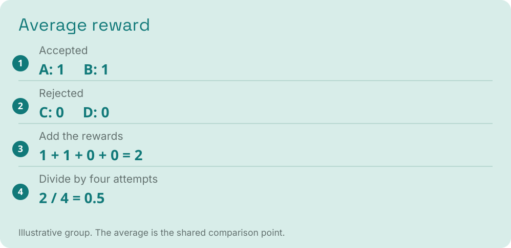
GRPO asks how each reward differs from that average. It divides these differences by the group's standard deviation, a measure of how spread out the rewards are. Dividing by the spread puts the differences on the same scale, even when one group has more varied rewards than another.
Walkthrough: the arithmetic below shows how to calculate that spread.
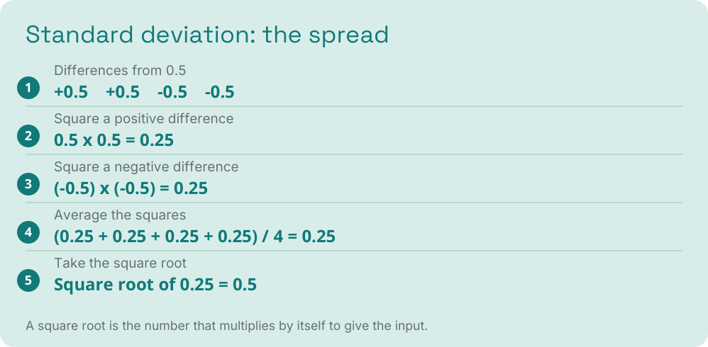
We are measuring all four rewards in this toy group, so the average of the squared differences divides by four.
Our four proofs earned 1, 1, 0 and 0. Their average and spread are both 0.5. Dividing each difference from the average by that spread gives its advantage, the score that tells training which proof to encourage.
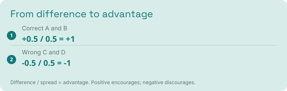
Positive means encourage this proof; negative means discourage it. Equal rewards within a group give no relative preference.
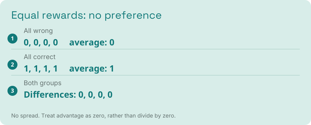
The actual training code handles this zero spread safely; the paper treats these groups as having zero advantage and skips their reward-driven updates.
To encourage a proof, training changes the model's weights, the numbers inside it that determine output probabilities.
It uses a gradient, a direction for changing those weights to improve the training score. Taking an update means moving the weights a small distance in that direction.
A gradient points toward a better training score. The picture separates that direction from the small step an update actually takes.
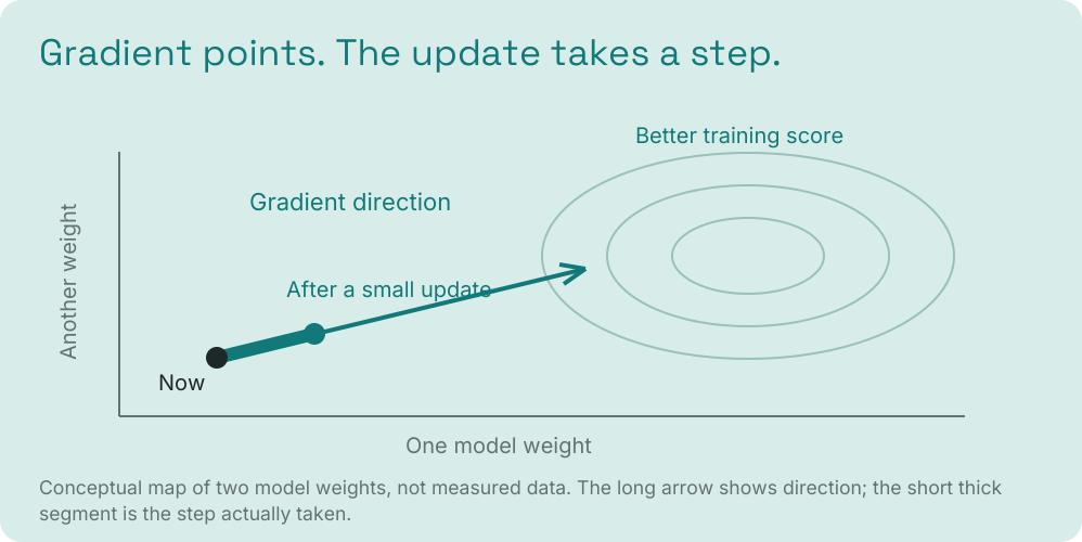
Training does not have a separate dial for each proof. The same internal numbers help produce many answers, so changing them to encourage one proof can also make other proofs more or less likely.
This is why a rare correct proof in a mixed group is interesting. It has a positive advantage. Yet that does not guarantee the shared weight update will make its probability increase. The paper measures the actual change, instead of assuming the positive score was enough.
Optional detail: How clipping limits the training incentive
Clipping, one step at a time
A positive advantage, the score comparing a proof's reward with its group, is encouragement rather than a promise. The optional panel explains clipping, a rule that limits how much an individual output contributes to pushing an update.
Teaching convention. The ratio below treats a whole proof as one action. The released language-model loss clips each generated token's probability ratio before combining them. It is not an exact whole-proof clipping implementation. Implementation source.
A batch is a collection of sampled attempts used together for training. Clipping compares two chances for the same proof: its old chance under the model that generated the batch, and its new chance under the model being updated. Divide the new chance by the old one. Call this ratio r.
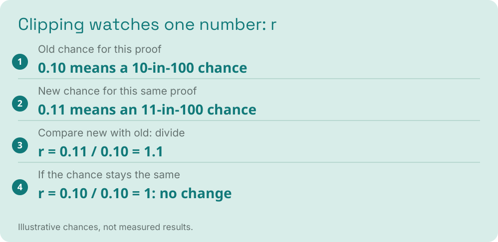
The ratio compares the new chance with the old one. A value of 1 means no change. Above 1 means the proof has become more likely; below 1 means it has become less likely.
The batch came from the old model, so pushing the new model too far based on those samples can make training unstable. Clipping removes the incentive for each proof to keep pushing a large change in the encouraged direction, helping training take more cautious steps.
Recall that r is the new chance divided by the old chance for the same proof. Clipping uses a chosen width called epsilon to make a band around r = 1. In the clipped score calculation, values outside this band become the nearest edge; values inside stay unchanged.
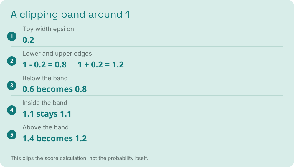
The training score, called the objective, takes the smaller of two scores: the ratio times the advantage, and the clipped ratio times the advantage. This deliberately less favorable choice removes the benefit of moving too far in the encouraged direction.
For a correct proof with positive advantage, once the upper limit is reached, making it even likelier earns no extra score from that proof.
Clipping is not a hard wall around the model's probabilities. It flattens one proof's contribution in one direction. Other proofs, shared weights and other terms in the objective can still move that probability. A later batch also has a new sampling model for its ratios.
GRPO builds on Proximal Policy Optimization, or PPO, an earlier reward-based training method. PPO usually trains a separate value model to predict expected reward as an answer unfolds, costing memory and training work. GRPO uses the group's average reward instead, removing that extra model. This makes it simpler to run, not better than every other RL method.
The objective also has a KL penalty. KL means Kullback-Leibler divergence, a measure of how differently two models spread chances across outputs. It discourages moving too far from a reference model, a saved comparison model. The final variants change this penalty too, so the reward alone cannot get all the credit.
Now we can return to the central question: does encouragement actually make a rare correct proof easier to find?
Why the usual training can miss a rare success
Now return to GRPO, the method that compares rewards within a group of attempts. A successful proof can receive a positive training signal relative to unsuccessful attempts.
That does not mean every successful proof becomes equally more likely. In the team's experiments, correct proofs that were already probable were more often reinforced than correct proofs near the unlikely end of the group.
They call this rank bias: the training outcome depends on where a proof sits in the model's probability ranking.
Probability here measures how likely the model is to generate that proof. Lean separately checks whether it is correct. A rare proof can be fully valid. A common proof can be wrong.
When training concentrates probability on familiar proofs, the result is distribution sharpening: more of the model's chances go to outputs it already tends to generate. It may become better at giving one correct proof while becoming less useful when we sample many proofs.
The clipping explanation from Spurious Rewards, my earlier coin-flip blog, only covers part of this problem. In Appendix E, the authors remove clipping in a controlled toy environment, a deliberately simplified setup for testing a mechanism. Rank bias still appears.
Unlikely correct proofs often do not increase in probability at all, rather than merely receiving a smaller increase. That leaves other causes to investigate alongside clipping.
The observation is that reinforcement varies with probability rank. The authors suspect the optimizer, the rule for changing model weights, contributes to this bias. That is a likely explanation, not a settled causal account. The no-clipping control rules out clipping as the only cause, not all other mechanisms.
Original paper Figure 4 below measures how often a correct proof's likelihood increased, from the familiar end of the sampled group to the rare end.
Optional detail: Figure 4, which correct proofs were reinforced
Figure 4: Which correct proofs became more likely?
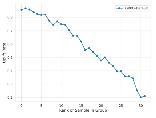
Original Figure 4. Horizontal axis: rank among 32 sampled proofs, from common to rare. Vertical axis: fraction of correct proofs whose probability increased after training. This is an uplift rate, not proof success. Original colours and axes preserved.
Figure: He, Fried and Welleck, Rewarding the Unlikely, EMNLP 2025
Keep the correct proof the model rarely chooses
What "rare" means in the code. A language model chooses tokens, small text pieces, one after another. A log probability is a score for how likely one choice is.
The released trainer averages these scores over a proof's tokens before ranking the group. This length-normalized likelihood can order short and long proofs differently from the probability of the entire proof. Here, "rare" is shorthand for a low score under that ranking.
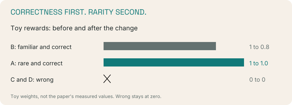
The reward change gives a rare correct proof more relative weight than a familiar correct proof. A wrong proof still gets zero.
Compare answers to the same question. The model often chooses one correct proof and rarely chooses another. Ordinary GRPO gives both the same reward: 1 point. The paper's change keeps more of that reward for the rare proof and reduces it for the familiar proof.
Think of a coach watching two valid ways to play the same ball. The player uses one all the time and almost never uses the other. The coach gives the less-used successful move more attention, to help keep it in the player's choices. A failed move still earns nothing.
The paper calls this the unlikeliness reward. It orders the sampled proofs by the likelihood measure just defined, then gives familiar correct proofs a bigger discount. This ranks answers to one question, not the difficulty of different questions.
In our example below, A is the rare correct proof and B is the familiar correct proof. C and D are wrong. The numbers illustrate the idea; they are not the paper's measured rewards.
A separate change: learn from the same attempts again
The reward change decides which correct proof counts more. The second change lets training use the same attempts again instead of collecting a new group. The paper calls each pass a PPO epoch. PPO means Proximal Policy Optimization, the training method GRPO builds on; an epoch here is one more pass over this batch.
The authors suggest why this helps: clipping limits an attempt's incentive to push a large update. Familiar proofs may reach that limit on the first pass, leaving rare correct proofs more influence on the next. Extra passes helped here, but cost more training time and can cause instability. They do not guarantee that every rare proof improves.
The final recipe combines both changes and increases a penalty for moving away from a reference model, a saved comparison model. We cannot give the reward change all the credit.
One limit on the reward change: if the original group is all correct or all wrong, it is skipped. The method still needs a correctness difference to learn from.
Optional detail: Adjusted rewards for our four proofs
Apply it to our four proofs
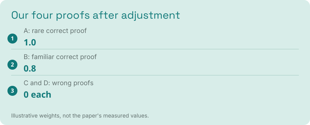
For our four proofs, we now say A is the rare correct proof and B is the familiar correct proof. C and D are still wrong.
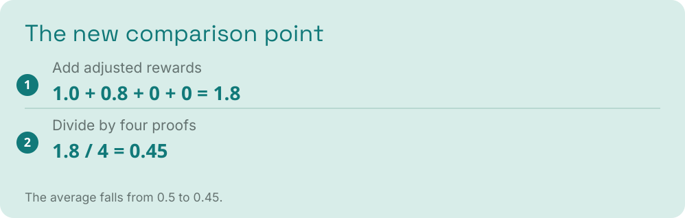
To compare these new rewards, first calculate their new average.
The rewards now differ, so we repeat the same group comparison with these adjusted values.
Optional detail: Recalculate the training signal
Walkthrough: repeat the same comparison
A is the rare correct proof, B is the familiar correct proof, and C and D are wrong. We divide by the new spread to put the new differences on the same scale. The takeaway is that A now gets stronger encouragement than B; the arithmetic below shows how.
This repeats the population-spread teaching convention from the first walkthrough. The released trainer's sample-spread correction changes the displayed advantage magnitudes, not which of these proofs gets the stronger signal.
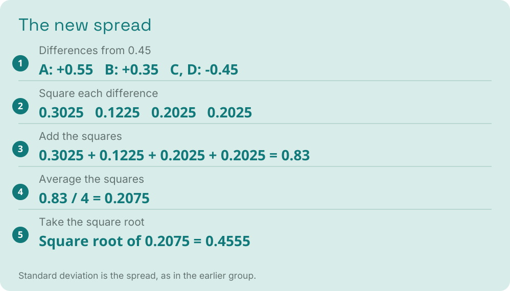
Now divide each difference from the average by this spread to get its advantage.
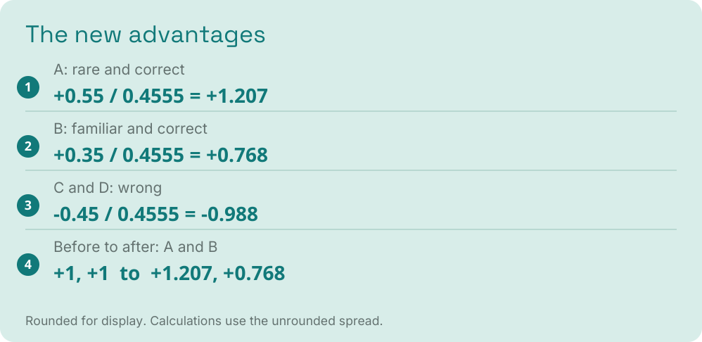
The rare correct proof now has a larger advantage relative to the familiar correct proof. Both still receive encouragement, and the wrong proofs still receive discouragement. This is a learning preference, not a guarantee that either proof becomes more likely.
Optional detail: Calculate the rank discount
What does 0.25 actually change?
The final recipe uses 0.25 as the reward-discount setting. It is not a flat 25% cut.
- Rank all sampled proofs for the same question, including wrong ones.
- Count the proofs below this proof in the implementation's likelihood ranking.
- Divide that count by the group size, multiply by 0.25, then subtract from 1.
- A correct proof receives that fraction of one point. A wrong proof receives zero.
For four proofs with different probabilities, the rule gives these values if the proof at that position is correct. The positions include wrong proofs too; this is not a ranking of correct proofs only.
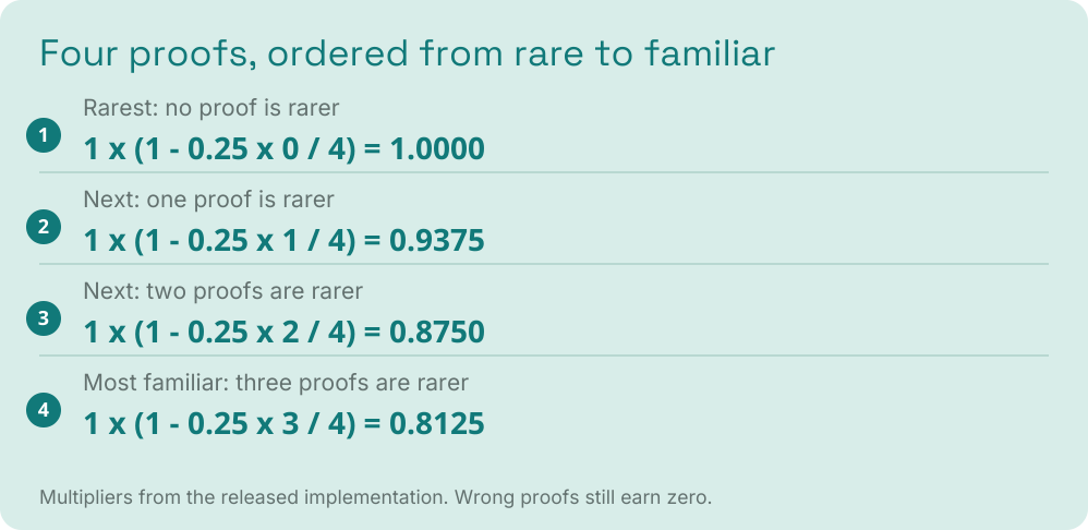
The rarest correct proof keeps 1 point. The most familiar correct proof keeps 0.8125 points: a cut of 0.1875, or 18.75%, not a flat 25% cut. The group size matters because the fraction changes.
Paper section 4.1 mixes rank conventions. This calculation follows the released trainer's _compute_advantages: ascending ranks 0 through G minus 1, divided by G. Checked at commit ca1cff05ebdf2cfe9737fd416897da838a93e11a.
The earlier A = 1.0 and B = 0.8 chart is a separate teaching illustration, not an exact calculation from this setting. The final recipe also uses two update passes and changes the reference-model penalty.
One try and several tries ask different questions
The diagnosis and the reward change matter only if they preserve useful chances to solve problems. We now compare one try with several tries before looking at the measured results.
The paper uses pass@N. Read it as: what fraction of problems receive at least one correct proof within N independently sampled attempts? Pass@1 is the one-attempt version. Pass@32 allows 32 attempts per problem. It is not the fraction of all 32 proofs that are correct.
A small made-up example shows why the distinction matters. "Independent" here means one random draw does not determine the next; it does not mean every generated proof has a different strategy.
Imagine an easy problem and a hard problem. Training improves the easy one but makes the hard one less likely to succeed on any single try.
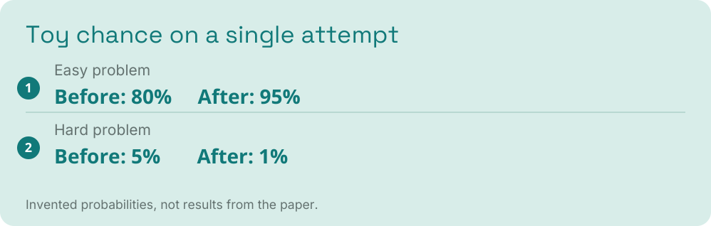
With one attempt per problem, their average success rises. With many independent attempts, the hard problem loses useful chances while the easy one has little room left to improve.
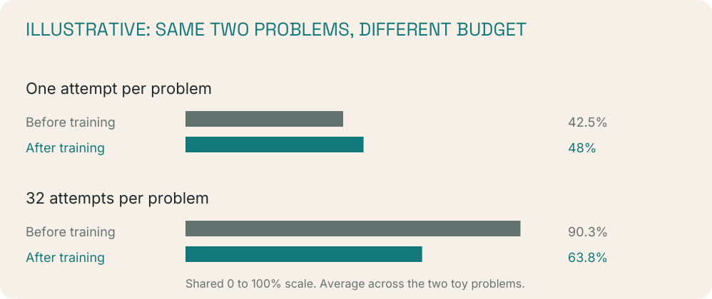
Training can raise the average first-try score while leaving fewer problems solved within 32 tries.
Illustration, not paper results: each try is sampled afresh with the same success chance. Fresh tries can repeat a proof; copying an earlier proof is not another chance. The two optional panels immediately below show the calculation.
Optional detail: Calculate success within 32 tries
Optional walkthrough: from one try to 32
Start with the hard problem from our toy example. Before training, a fresh attempt succeeds 5% of the time. After training, it succeeds only 1% of the time. These are invented chances, not paper results.
We want the chance of at least one success in 32 attempts, not 32 successes. The easiest route is to find the chance that all 32 fail, then subtract it from 100%.
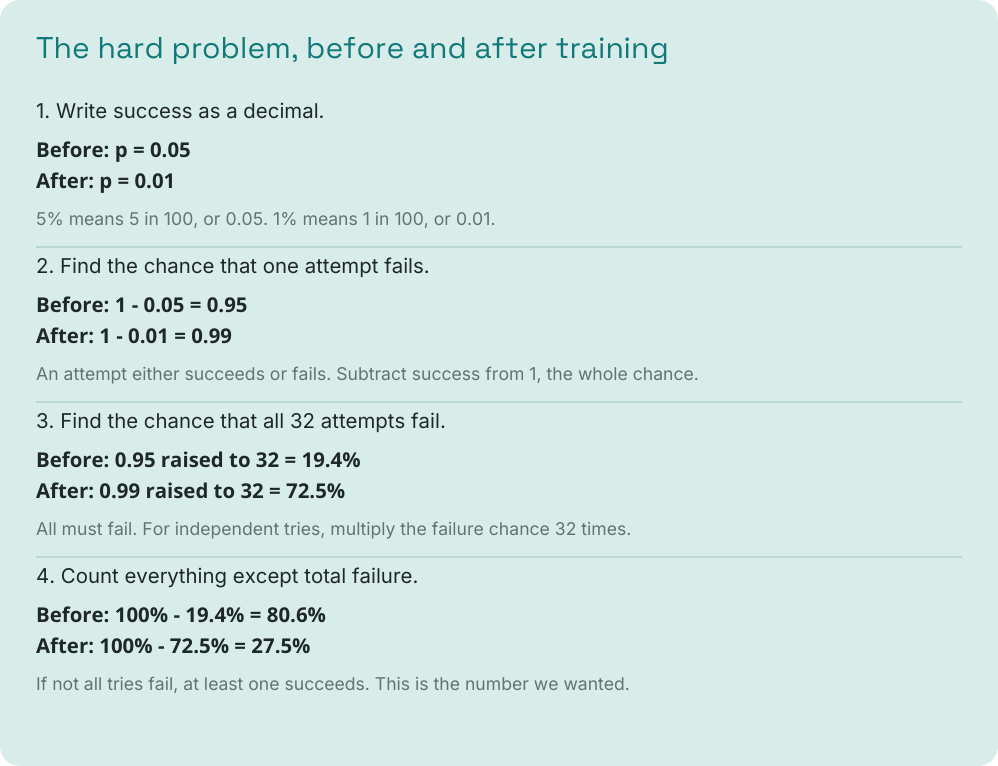
The general rule is 1 − (1 − p) raised to N. Here p is the one-try success chance written as a decimal, and N is the number of tries. "Raised to N" means multiply the same number by itself N times.
This assumes each attempt is a fresh, independent draw with the same success chance. Independence means one result does not change the next attempt's chance. Repeating a stored answer is not a fresh draw. New draws can still produce the same proof.
Optional detail: Calculate the easy and hard average
Optional walkthrough: compare the easy and hard problems
The bar chart gives equal weight to two problems: one easy and one hard. Before training, their one-try chances are 80% and 5%. After training, they are 95% and 1%. We average the two problem-level chances to get each bar.
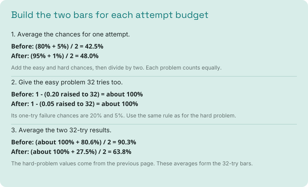
Why can the two budgets tell opposite stories? With one try, the easy problem's gain outweighs the hard problem's loss. With 32 tries, the easy problem is already almost certain to be solved in either case. Its improvement adds almost nothing, while the hard problem's loss remains large.
The point is not that more attempts hurt. For each version of the model, 32 tries beat one. The point is that training looks better at one try and worse at 32 in this example.
This average is an expected fraction of the two problems solved, not the chance that both are solved. The easy-problem values round to 100.0%; neither is exactly 100%. All displayed results are rounded, and the averages use the unrounded values.
What the experiments actually show
The authors do not start from scratch. They use DeepSeek-Prover-V1.5-SFT, a model already trained on example proofs. SFT stands for supervised fine-tuning: learning from examples of correct proofs. Now they ask what training with rewards changes.
They keep separate validation problems to compare training choices. These problems do not supply training updates, but repeated use can influence which recipe is chosen. Validation is not the same as an untouched final test.
The final comparison asks what the combined recipe adds to a model that already writes proofs. It lines up three models:
- Example-trained start: DeepSeek-Prover-V1.5-SFT, before reward training.
- Existing reward-trained model: DeepSeek-Prover-V1.5-RL, released in earlier work. This is not the ordinary-GRPO curve in Figure 5.
- Combined recipe: the new reward and two update passes, with a changed reference-model penalty.
Does the combined recipe solve more problems?
Each model gets up to 128 tries per problem. A problem counts as solved if at least one proof passes the checker. Each percentage below is the share of problems solved, not the share of individual proofs that pass.
The combined recipe means the adjusted reward plus two update passes, with a changed penalty for moving away from the saved comparison model. The two collections test it on different problems.
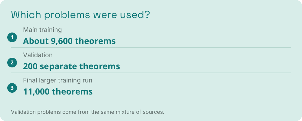
The 200 validation problems come from the same mixture of sources as the main training set, but never supply training updates. The second collection, miniF2F-test, is a separate collection used to compare proof-writing models. F2F means formal-to-formal: a computer-readable mathematical claim goes in and a checked proof comes out.
| Model | 200 validation problems | miniF2F-test |
|---|---|---|
| Example-trained start | 83.1 ±0.2% | 49.2 ±0.6% |
| Existing reward-trained model | 87.5 ±0.7% | 51.2 ±0.3% |
| Combined recipe | 88.8 ±0.9% | 50.6 ±0.5% |
Source: paper Table 3. ± is standard deviation across sampled evaluation chunks, not a confidence interval or variation across training seeds. Same 128-attempt limit; no claim of matched training cost.
Higher on validation, not higher everywhere. The combined recipe reaches 88.8% on validation, compared with 87.5% for the existing reward-trained model. On miniF2F-test, it reaches 50.6%, below that model's 51.2%.
These are averages across repeated evaluations using different groups of sampled proofs, not proof that one model wins reliably. The paper reports variation across those evaluations too. Close scores do not establish a clear overall winner.
The table shows only 128 tries. The separate experiment in Figure 5 compares attempt budgets: the modified reward trades a little success at one or two tries for more success at larger budgets, compared with ordinary GRPO. That curve is not a head-to-head comparison with the existing DeepSeek reward-trained model above.
The contribution is a diagnosis and an open training recipe, meaning the training code is available for others to inspect and use.
Does ordinary training still help after many tries?
Ordinary GRPO helps most when the model gets few tries. On these validation problems, that gain shrinks and turns into a loss at larger attempt budgets.
Optional detail: Figure 2, ordinary training across attempt budgets
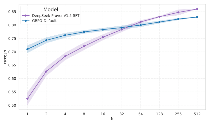
Original Figure 2. On the 200 validation theorems, ordinary GRPO (blue) beats the supervised starting model (purple) with few attempts, but falls behind at larger budgets. The horizontal axis is attempts per theorem; the vertical axis is the fraction solved at least once. The paper calls this validation set Dval. This is measured data, unlike our two-problem illustration.
Figure: He, Fried and Welleck, Rewarding the Unlikely, EMNLP 2025
What changes when rare successes count more?
The adjusted reward and extra update passes improve success at larger budgets in these comparisons. The reward version gives up a little at one or two tries; extra passes cost more training time.
Optional detail: Figure 5, compare the training variants
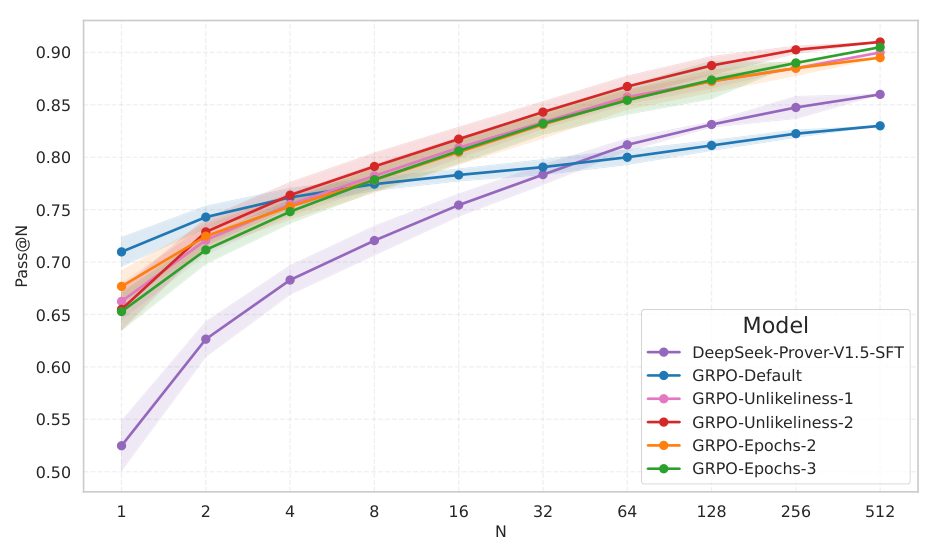
Original Figure 5. Each curve shows the fraction of the 200 validation theorems solved with at least one success within N attempts. N doubles along the horizontal axis; it is not a linear attempt scale. SFT is the supervised starting model, Default is ordinary GRPO, Unlikeliness changes the reward, and Epochs changes update passes. Original colours, legend and axes preserved.
Figure: He, Fried and Welleck, Rewarding the Unlikely, EMNLP 2025
Do rare correct proofs become easier to find?
The combined recipe is more likely to reinforce the rare end of the sampled group. Extra passes also help. Because other settings change, this does not isolate the reward's effect.
Optional detail: Figure 6, reinforcement from common to rare
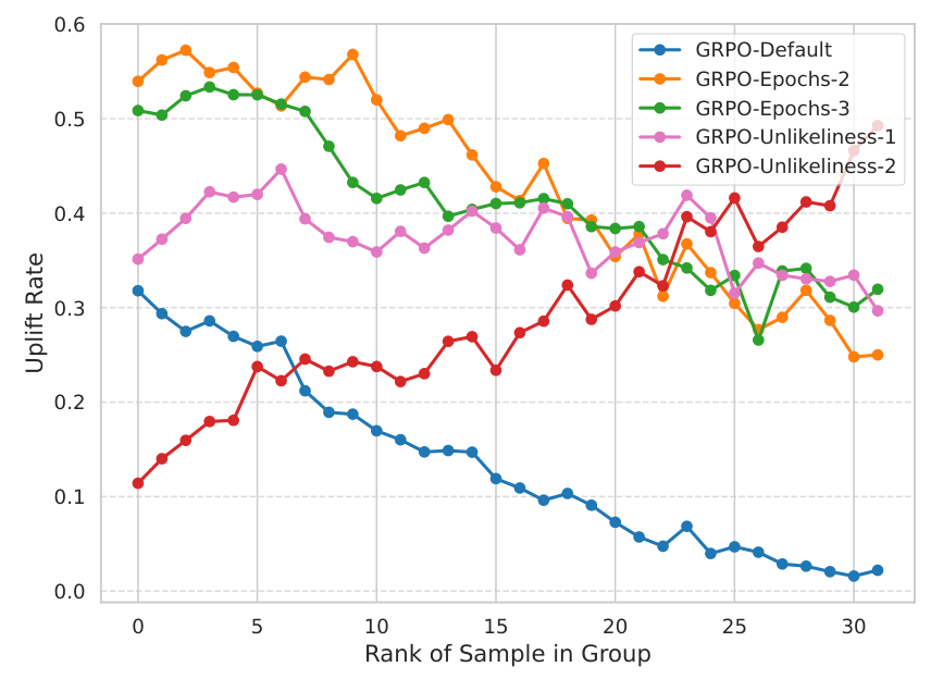
Original Figure 6 compares training variants. The horizontal axis orders sampled proofs from common to rare.
The vertical axis is the fraction of correct proofs whose chance increased, not the fraction solved. Ordinary GRPO (blue) rarely reinforces the rare end. The combined adjusted-reward, two-pass recipe (red) reverses that pattern. Extra passes without the reward change (orange and green) help too. These variants also change the reference-model penalty, so this is not evidence for the reward alone.
Figure: He, Fried and Welleck, Rewarding the Unlikely, EMNLP 2025
Does training keep different proofs available?
The combined recipe's count of distinct proof outputs first falls, then recovers. Ordinary GRPO keeps losing variety in this run. Distinct text alone does not establish different useful strategies.
Optional detail: Figure 7, proof variety during training
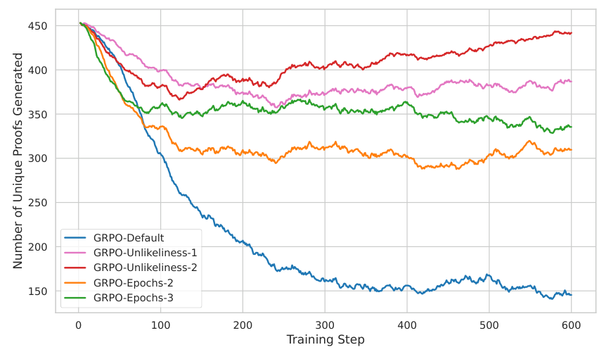
Original Figure 7 counts distinct proofs produced at each training step. A training step is one round of generating proofs and training on that batch.
The horizontal axis tracks training; the vertical axis counts unique proofs. The combined two-pass adjusted-reward recipe (red) initially loses variety, then recovers. Ordinary GRPO (blue) keeps losing variety. The lines are smoothed, meaning nearby measurements are blended to make the trend clearer. More unique text is not automatically more useful correct approaches.
Figure: He, Fried and Welleck, Rewarding the Unlikely, EMNLP 2025
My proposed test: start with code generation
My proposed test moves this idea from formal proofs to code generation. One attempt produces a complete Python program for a fixed input/output task, not a multi-step coding agent. The question is whether rare, checked approaches help solve more tasks at the same total cost.
This has not been run. Tests provide evidence, not a proof of correctness on all inputs. A later coding-agent experiment would also need to define tool actions, environment resets and the likelihood of a whole action sequence.
Optional detail: Models and training controls
- Start from one fixed code model. Pick and freeze the task set, model checkpoint and sampling settings before training. These choices are not selected yet.
- Compare no additional training, ordinary GRPO, reward discount only, extra passes only, both changes, and a stronger-KL-only control. KL is the reference-model penalty. Hold it fixed across ingredient comparisons; use the extra control to isolate its effect.
- Include filtered supervised learning, which trains on successful generated programs without reward updates. Also compare the same untrained model with sampling and a fixed number of repairs using visible-test feedback. Charge that inference work to its budget.
Optional detail: Scoring and hidden-test separation
At 1, 4, 16 and 32 candidates, report oracle pass@N: the share of tasks for which at least one program passes hidden evaluation tests. "Oracle" means we can inspect every candidate after generation. Also report selected-program success: the share of tasks where the single program returned by a fixed selector passes those tests.
The selector first filters candidates using visible tests, then picks the surviving candidate with the highest length-normalized model likelihood. No survivor means failure. Freeze that rule across variants. Hidden evaluation tests never enter training feedback, repair, ranking or selection.
Training rewards use a separate training-only verifier. Hidden evaluation tests stay sealed until scoring. Run generated code in a sandbox with no network or secret access, a disposable filesystem, and fixed time and resource limits. A separate process alone is not enough isolation.
Optional detail: Cost accounting and mechanism checks
Use a fixed price for each resource. A text token is a small piece of generated text; processor time measures how long the machine works.
- Freeze prices before the run. Track training-processor time, generated text tokens and test-processor time separately.
- Compare quality at matched dollar budgets under those prices. Include generation, verification, updates, judge fees and repairs.
- Extra update passes must buy fewer batches or consume a larger budget. Show the tradeoff rather than calling equal tries equal compute. Charge any judge and repair work too.
- On a fixed held-out set of correct programs, measure before/after length-normalized likelihood uplift by initial rank. This tests whether initially rare correct candidates are actually reinforced, alongside tasks solved.
- Textual variety is not strategy variety. Human reviewers label a small fixed sample for substantive algorithmic differences, with uncertain cases kept separate. Extra variable names do not create a new strategy.
Optional detail: Judge limits and links to agent research
Jev, TypeSafe AI's typed-verdict model, returns one of the labels you specify with a confidence score. It is an optional triage hypothesis, not an established code judge.
Its published evaluation finds weaker results on difficult coding judgments than its strongest comparator. Test its approach and shortcut labels on human-reviewed code first, freeze the confidence cutoff and count judge cost. Execution and hidden tests determine the scored correctness outcome; judge confidence cannot overrule a failure.
Fried's Scaling Test-Time Compute for Agentic Coding makes selection and reuse of rollout experience explicit. His coauthored Hybrid-Gym tests coding-skill transfer across task types. Those are relevant comparisons for a later agent experiment, not evidence that this proposed reward change already works for agents.
A test card to keep
- Freeze the starting model, tasks, public checks, sampling settings and the rule that selects one output.
- Compare the reward change alone, extra training passes alone and both together. Keep the penalty for moving from the reference model fixed.
- Measure both tasks solved by any candidate and tasks solved by the single selected output. Include sampling, repair and successful-example training as controls.
- Count training, generation, checks and repairs in the cost. Check whether initially rare correct programs become easier to generate.
- Keep hidden evaluation checks out of feedback and selection. Use human-reviewed examples to distinguish new approaches from renamed variables.
- If the benefit disappears on hidden tasks, selected outputs or matched-cost comparisons, narrow or drop the claim.
Proposal, not a result. The task set and checkpoint still need selection. This is a testable code-generation design, not a completed experimental protocol or a demonstrated coding-agent improvement.
Previously covered, and what is different here
These posts share a question: how do we get useful answers? This paper adds another: once a correct answer appears, does training keep it available? None of the earlier posts is required reading.
| Earlier post | Earlier focus | This paper |
| Spurious Rewards: the coin flip | reinforcing familiar habits | diagnosing overlooked rare successes |
| Never Give Up and Day 4 | finding answers with more tries | keeping found answers within reach |
| The one percent | prioritising hard cases (my proposal) | rewarding rare correct proofs (tested) |
| Beyond Repeated Sampling | guiding the search with strategies | training on successful answers |
| Progressive Point Matching | rewarding useful intermediate steps | adjusting rewards for correct proofs |
| MAHALO: multiple rewards | balancing several goals | varying rewards among correct proofs |
| GRPO: tool use | checking tool use strictly | testing what strict feedback preserves |
Finding an answer is one job. Checking it is another. This paper asks whether training keeps it available for the next attempt.
Paper: https://aclanthology.org/2025.emnlp-main.1298/
Implementation: https://github.com/AndreHe02/rewarding-unlikely-release
Research agenda: https://dpfried.github.io/
Optional detail: Implementation sources
Implementation conventions: reward ranking and spread; token-level policy loss. Paper evidence: equations 1 and 2, sections 3.5 and 4.1, Table 3, Appendices C to E.
In short
- Measured: reward training can overlook rare correct proofs. The combined recipe helps at larger attempt budgets in these experiments, but it changes several settings and is not better on every benchmark.
- Limits: extra updates and attempts cost more. Different proof strings do not necessarily mean different strategies.
- Proposed, not tested: compare code-generation variants on hidden tasks, selected outputs and matched costs.
Takeaway: finding a correct answer and training the model to find it again are different jobs.